この節の作者: Sebastian Jentschke, Rebecca Vederhus
From SPSS to jamovi: Logistic Regression
This comparison shows how a binary logistic regression is conducted in SPSS and jamovi. The SPSS test follows the description in chapter 20.5 - 20.6 in Field (2017), especially figure 20.7 - 20.10 and output 20.1 - 20.5 (bootstrap excluded). It uses the data file Eel.sav which can be downloaded from the web page accompanying the book.
| SPSS | jamovi |
|---|---|
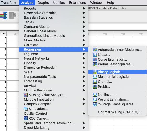
In SPSS you can run a binary logistic regression using: Analyze →
Regression → Binary Logistic. |
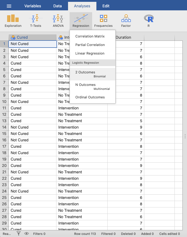
In jamovi you do this using: Analyses → Regression → 2 Outcomes
Binominal. |
 |
 |
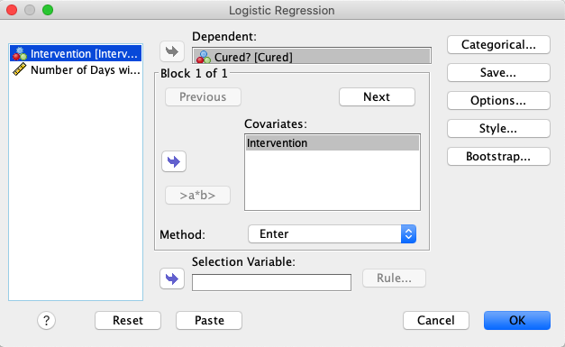
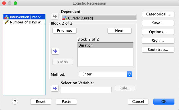
In SPSS, move Cured to the Dependent variable box and
Intervention to the Covariates variable box. |
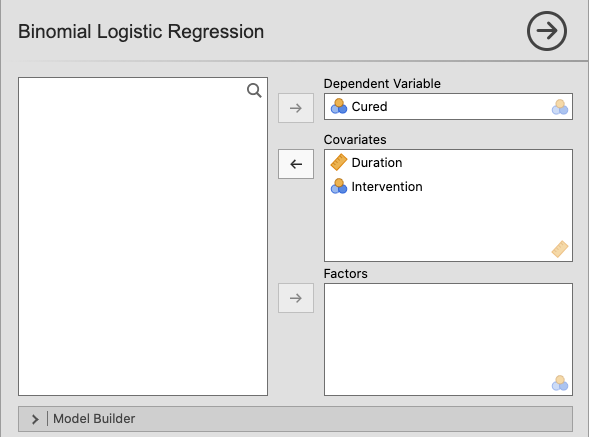
In jamovi, move the variable Cured to Dependent Variable and the
variables Duration and Intervention to Covariates. |
 |
 |
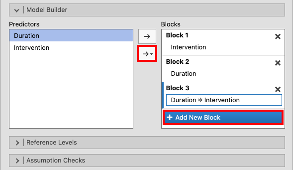
Click Next and add Duration to this new block. |
Create two new blocks by clicking + Add New Block in the Model
Builder drop-down menu. Add the Duration variable to Block 2, and
add Duration and Intervention to Block 3 by marking them both and
clicking Interaction in the drop-down menu. |
 |
 |
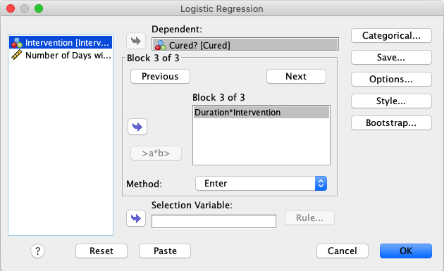
Create a third block by clicking Next one more time, and create an
interaction by marking both Intervention and Duration and moving
them to the block by pressing the arrow. |
|
 |
|
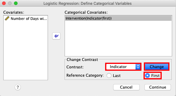
Access the Categorical window and open the drop-down menu for
Contrast. Here, choose Indicator and then check First as the
Reference Category. Click Change. |
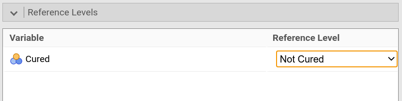
jamovi set the reference category automatically to the first category. If you
were to change that, open the drop-down menu Reference levels, and change
the reference level for each variable to the desired level (e.g., Not
Cured). |
 |
 |
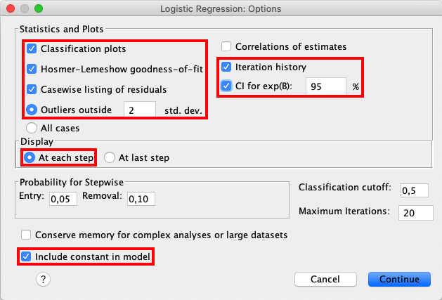
Open the Options window and check the following boxes: Classification
plots, Hosmer-Lemeshow goodness-of-fit, Casewise listing of
residuals, Outliers outside 2 std. dev., Iteration history,
CI for exp(B), At each step, and Include constant in model. |
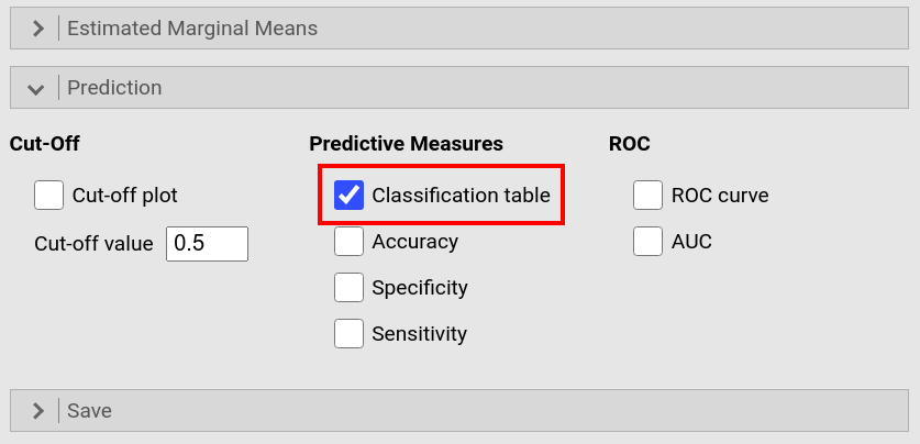
Open the drop-down menu Prediction and tick Classification table. |
 |
|
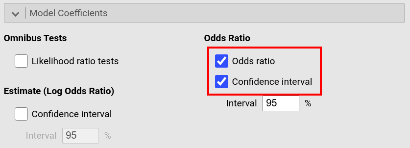
In the drop-down menu Model Coefficients, tick Odds ratio and the
Confidence interval to odds ratio. |
|
 |
|
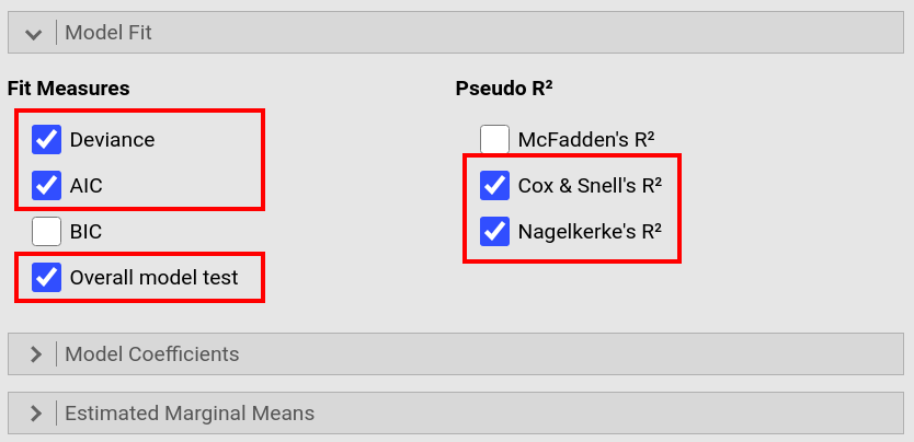
In the Model Fit window, check the boxes for Deviance, AIC,
Overall Model Test, Cox & Snell's R² and Nagelkerke's R². |
|
 |
 |
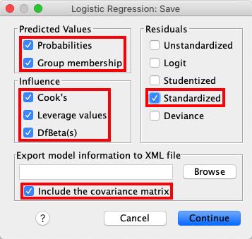
Open the Save window and check Probabilities, Group membership,
Cook's, Leverage values, DfBeta(s), Standardized (residuals),
and Include the covariance matrix. |
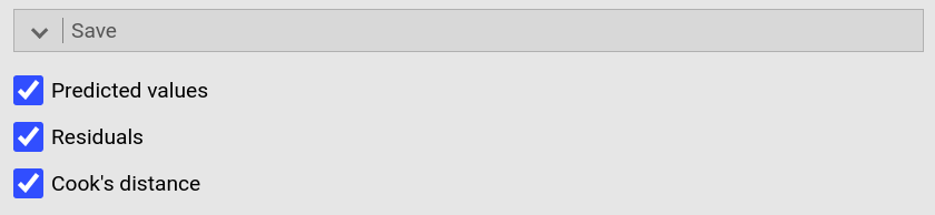
jamovi permits you to save some of these values too. To do so, open the
drop-down menu Save and tick Predicted values, Residuals, and
Cooks's distance. |
 |
 |
| If you compare the output from SPSS and jamovi, the results are essentially the same. However, the results from jamovi are shorter and better structured, whereas the SPSS results are much more extensive (likely to the more comprehensive choice of options, according to Field, 2017). jamovi, furthermore, first has an overview over the models and their comparison whereas SPSS provides those model indices within each model. | |
 |
|
 |
 |
 |
 |
 |
 |
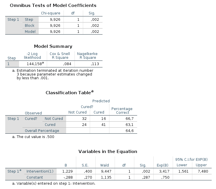
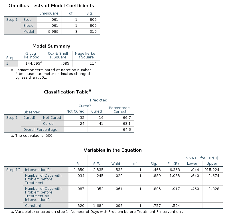
In the output from SPSS you can find tables for Model Summary,
Variables in the Equation and Omnibus Tests of Model Coefficients for
each of the predictors in the model. The Model Summary tables shows the
-2LL value for the model, as well as Cox & Snell R² and Nagelkerke R². In the
Omnibus Tests of Model Coefficients tables, χ²-values, degrees of freedom
and significance values are found. Lastly, you can find b-values,
SE-values, degrees of freedom and significance values in the Variables in
the Equation table. This table also shows the odds ratio. |
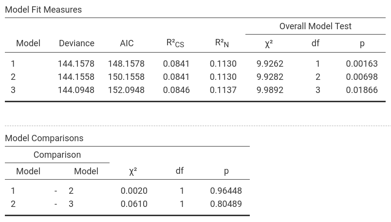
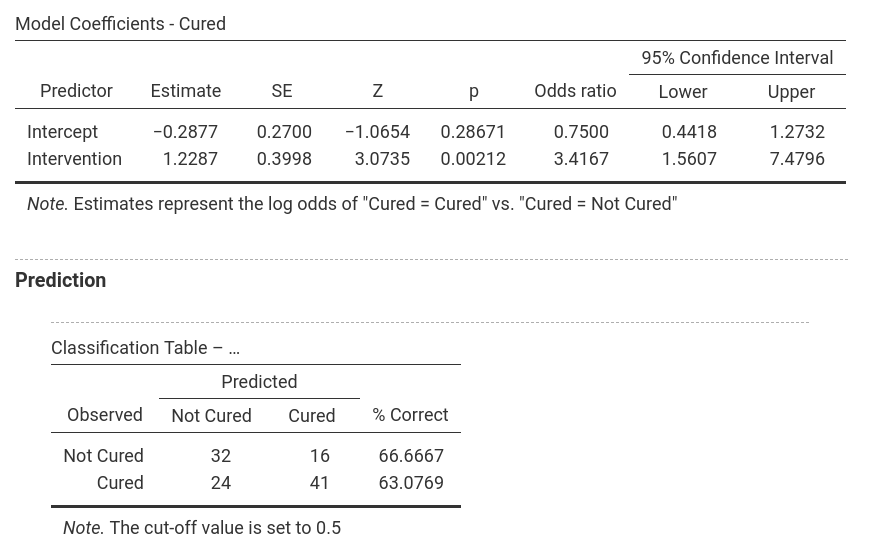
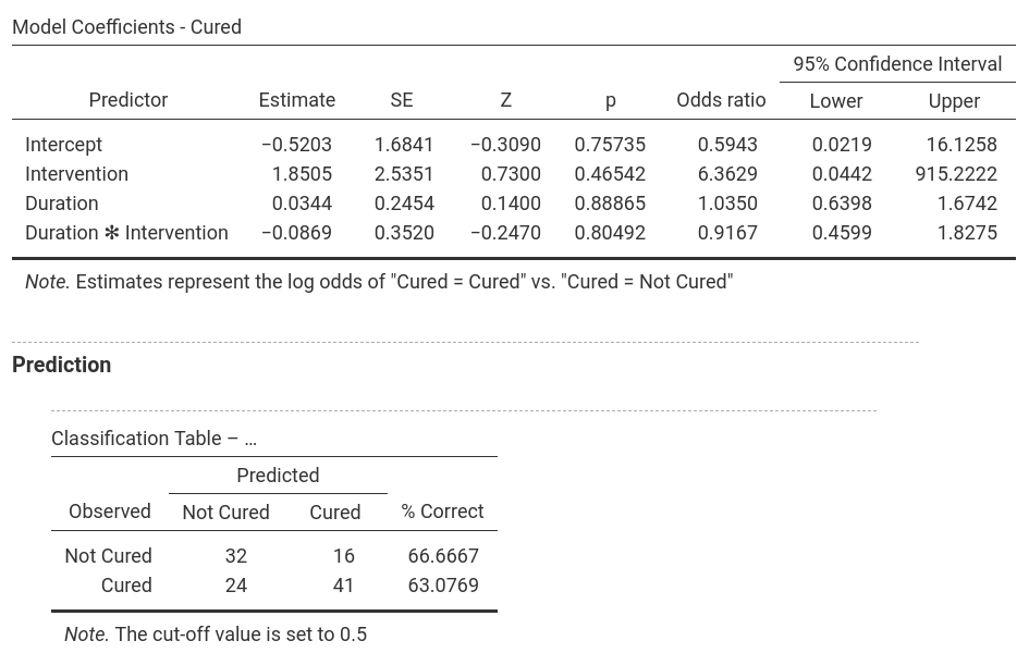
In jamovi, -2LL values, Cox & Snell R² and Nagelkerke R² values for all the
predictors are found in the table called Model Fit Measures. χ²-values,
degrees of freedom and significance levels are found in the Model
Comparisons table. In addition, b-values, SE-values, significance level
odds ratio and the confidence interval for it as well as the classification
table are shown as separate parts of the output (one for each model). Only
one model is shown at a time and the model can be selected by using the
drop-down menu next to Model Specific Results. |
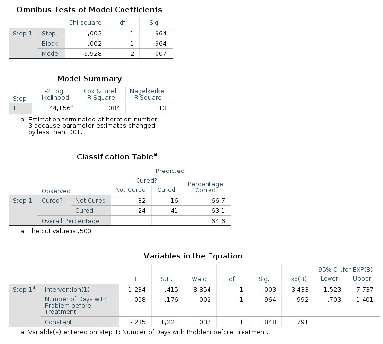
SPSS produces a lot more output tables (some not shown) than jamovi, not the least due to Field (2017) asking for options that are not available in jamovi.
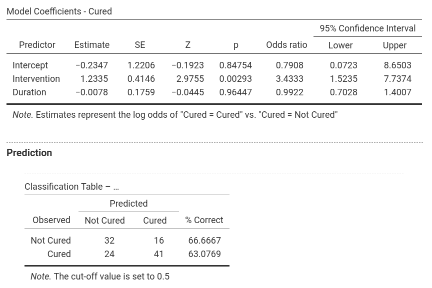
The numerical values for the results are the same.
Model 1: -2LL = 144.158, χ² = 9.926, df = 1, p = 0.002, R²CS = 0.084, R²N = 0.113, corr.NC = 66.667, corr.C = 63.077
Model 2: -2LL = 144.156, χ² = 9.928, df = 2, p = 0.007, R²CS = 0.084, R²N = 0.113, corr.NC = 66.667, corr.C = 63.077
Model 3: -2LL = 144.095, χ² = 9.989, df = 3, p = 0.019, R²CS = 0.085, R²N = 0.114, corr.NC = 66.667, corr.C = 63.077
It becomes clear that
Intervention is the most decisive predictor whereas Duration and the interaction of Intervention × Duration don't really
lead to better prediction: The number of correctly classified cases doesn't change between the models while Model 1 is the most parsimonuous; furthermore,
the Deviance (-2LL) and χ² for Model 2 and 3 are more or less the same as for Model 1 (and since more df's are used in Model 2 and 3, the p-values increase
(which is all emphasizing that Model 1 is the best model and should be selected). |
|
| If you wish to replicate those analyses using syntax, you can use the commands below (in jamovi, just copy to code below to Rj). Alternatively, you can download the SPSS output files and the jamovi files with the analyses from below the syntax. | |
LOGISTIC REGRESSION VARIABLES Cured
   /METHOD=ENTER Intervention
   /METHOD=ENTER Duration
   /METHOD=ENTER Duration * Intervention
   /CONTRAST (Intervention)=Indicator(1)
   /SAVE=PRED PGROUP COOK LEVER DFBETA ZRESID
   /CLASSPLOT
   /CASEWISE OUTLIER(2)
   /PRINT=GOODFIT ITER(1) CI(95)
   /CRITERIA=PIN(0.05) POUT(0.10) ITERATE(20) CUT(0.5).
|
jmv::logRegBin(
    data = data,
    dep = Cured,
    covs = vars(Duration, Intervention),
    blocks = list(list("Intervention"),
                  list("Duration"),
                  list(c("Duration", "Intervention"))),
    refLevels = list(list(var="Cured", ref="Not Cured")),
    pseudoR2 = c("r2mf", "r2cs", "r2n"))
|
| SPSS output file containing the analyses | jamovi file containing the analyses |
References
Field, A. (2017). Discovering statistics using IBM SPSS statistics (5th ed.). SAGE Publications. https://edge.sagepub.com/field5e